Data retrieval
This page describes the functions of the Data retrieval web application. With this web application you can retrieve HiSPARC data, with which you can make plots.
Here is a step by step guide for the functions of the page.
Get data
The page will be quite empty at first and only show the HiSPARC logo and two forms with which you can either download data or load local datafiles. Whenever the HiSPARC logo becomes animated, it indicates that data is being retrieved from the HiSPARC servers.
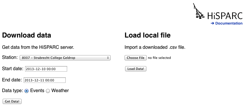
The two forms to load data and the HiSPARC logo indicating activity.
Download data
If you choose to download data you can first select a HiSPARC station, the start and end date (and time) and the type of data you want to get. Once you have made your choices click Get Data!.
Local data
If you already have a .tsv file (tab-separated values) on your computer, you can load that into the web application. The application will try to interpert the filename of the .tsv the following way: [data type]-s[station number]-[start date]_[end date]. If the data type is one of the types provided by the HiSPARC Public Database the web application tries to identify the columns, otherwise it will simply give each column a number.
Data overview
Once the data has been (down)loaded a new section on the website appears, giving you and overview of all the datasets that you have. It is possible to get multiple datasets, simply use the form again to get another.
For each downloaded dataset you can see the options that were used in the form, the number of entries it contains. Each row also has controls to choose, preview, download and remove a dataset.

An overview of the loaded datasets.
Controls
Here you can choose which datasets you wish to use for creating plots by selecting them in the Choice columns. The Preview button creates a table overview of the dataset. The Download button downloads the dataset as a .tsv file (tab-separated), which can be imported in other applications like Excel. Finally there is a Remove button, this simply removes the dataset from the browser memory.
Plot options
Once you have chosen at least one dataset (with the Choice column) the plot controls appear, with which you can select the type of plots you want to create: Scatter, Histogram or a Time series. You can also choose whether to display the x and y axes as linear or logarithmic and the number of bins for the histogram plot.
To the right of these options are the available variables from the chosen dataset, you can choose which variable to use for the x, and which to use for the y-axis. After selecting a plot type which requires only one variable, the other axis column will be disabled. For instance a histogram requires only x-axis values, the y-axis values are the number of counts in each bin, so the y-axis selection will be disabled.
Once you have made your choices you can click the Create Plot button and the plot will be shown in a new section appearing under these options. If you wish to create a different plot, simply change the options and click Create Plot button again.
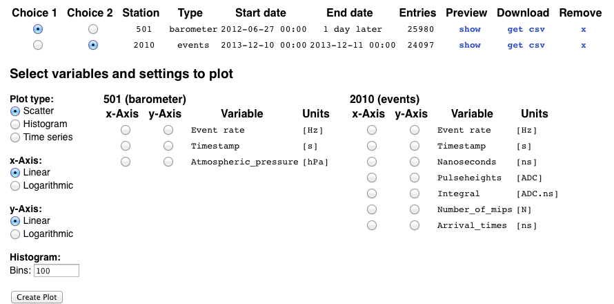
Options for creating plots and variable lists to select which variables to plot.
Interpolation
It is possible to get multiple datasets and then select one dataset as choice 1 and another as choice 2. When two datasets are chosen the variables for each dataset will appear side by side, and variables for the x or y axes can be chosen from either dataset. If the x and y data are from different datasets the data will be interpolated to match the different timestamps. This can cause strange values in some cases, especially when the start and end dates for the two datasets do not match.
Plot
The plot view appears as soon as you click Create Plot. On the top right is a Save image button that will open a new window with a .png version of the plot, which can be saved to your pc. Currently there are no options to change axis limits (zoom in, move around).
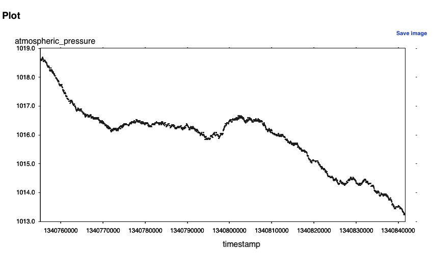
An example plot of barometer data.
Data preview
If you click the show button for a dataset this section will show a table with some rows of data. Each row shows all variables in the dataset for each event. At first a small subset will be shown, since it would take the browser to long to display all data rows. You can shows more by clicking the line in the middle of the shown data. However, if you wish to see all data, it is better to download the data to your pc.
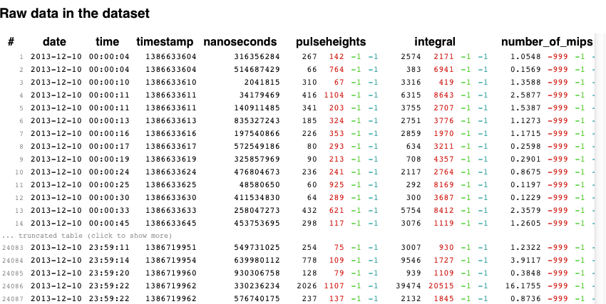
The data preview table showing the raw values in the dataset.
Event traces
Cosmic-ray events consist of signal measurements from each PMT with a scintillator detector. Variables like Pulseheight and Arrival time are derived from these signals. These signals are referred to as traces. When looking at the data for a cosmic-ray dataset the last column is called Traces and will contains show buttons for each event. When clicked, the traces are retrieved and them shown in the plot.
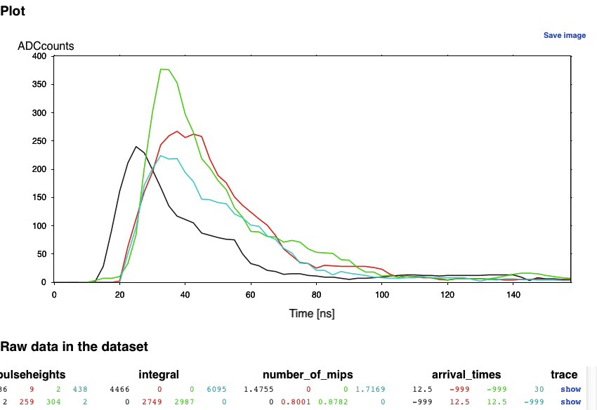
The traces of a chosen event.
Multiple detectors
Depending on your choice of variables a plot may contain datapoints with multiple colors, this is because some variables are measured by multiple detectors. For cosmic-ray data there are either 2 or 4 detectors for the Pulseheights, Integral, Number of mips and Arrival times, the colors are respectively black, red, green and blue. For weather data the Temperature and Humidity are measured both indoor (black) and outdoor (red).
Missing data
When a weather sensor is out of duty or a cosmic-ray station has 2 detectors instead of 4, the missing data will be given the value -999 or -1. Those error values are omitted in the plot, preventing distortions of the plot limits. A problem can arise when working with temperatures that include -1 °C, because the filter will remove it, though it is a valid measurement. Luckily a temperature of -1 °C is fairly rare.