Tutorial

SAPPHiRE simplifies data access, simulations and analysis for the HiSPARC experiment. In this tutorial, we’ll try to give you a feeling for the things you can do with SAPPHiRE. How can you download data? How can you analyze this data? How can you produce pulseheight histograms? How can you calculate the direction of cosmic rays? This tutorial will only give you an overview of what’s possible with SAPPHiRE. For details on all available classes and methods, please see the SAPPHiRE Reference.

Note

We’ll require you to know basic Python. If you’re unfamiliar with Python, you can look at the official Python tutorial, the book Think Python, or Getting started with Python for science.

First steps

In a few examples, we will plot the data which we have produced. We make use of pylab, which is included with matplotlib. If you have Anaconda installed, you can use the Spyder environment. You can write a script in the main window, or type short commands in the command prompt in the bottom right. The first thing you have to do is import everything from pylab. That makes it ridiculously easy to plot things:

>>> from pylab import *

You can also start an IPython terminal with pylab using:

$ ipython --pylab

In that case, you don’t need to import pylab.

Whenever you see something like:

>>> print('Hello, world')
Hello, world

it means we’re typing in Python code. The >>> is the Python prompt. It tells you that the Python interpreter is waiting for you to give it some instructions. In the above example, we’ve typed in print ('Hello, world'). The interpreter subsequently executed the code and printed Hello, world on the screen.

The first thing we’ll have to do to start using SAPPHiRE is to import the SAPPHiRE module:

>>> import sapphire

There will be no output if everything is succesful. It is easy to get some help from inside the Python terminal. Just say:

>>> help(sapphire)

and you’ll be presented with a basic help screen. Instead of sapphire, you can throw in modules, packages, functions, classes, objects, etc. Everything in Python has some help text associated with it. Not all of it is very helpful to a newcomer, hence this tutorial. All help text is also available in the SAPPHiRE Reference.

Downloading and accessing HiSPARC data

The SAPPHiRE package comprises multiple modules and packages. To access data from the public database, we’ll have to import the sapphire.esd module. This module gives us access to the event summary data, which is the raw HiSPARC data with preliminary analysis already included. It is simple to quickly start playing with data:

>>> from sapphire import esd
>>> data = esd.quick_download(102)
100%|####################################|Time: 5.91
>>> print(data)
data8.h5 (File) ''
Last modif.: 'Thu Oct 22 16:02:05 2015'
Object Tree:
/ (RootGroup) ''
/s102 (Group) ''
/s102/events (Table(46382,)) ''

First, we import the sapphire.esd module. Then, we download data from station 102 using the sapphire.esd.quick_download() function. This function downloads yesterday’s data, and creates a datafile on the fly. More on that later.

If we want to exercise more control, we need to do some things manually. First, we need the tables module to actually store the data. PyTables is based on the open HDF5 data format, which is used by many (research) institutes. For example, it is used by the KNMI and by NASA. To specify the date and time for which to download the data, we need the datetime module. Thus, we have:

>>> import tables
>>> import datetime
>>> from sapphire import esd

Creating an empty data file, with the name mydata.h5, is done easily:

>>> data = tables.open_file('mydata.h5', 'w')

The 'w' means write, which creates a file for writing (and reading). Mind that this will create an empty file. If there already was a file with that name, it will be overwritten! Alternatively, you can say 'a', which means append, thus adding to an existing file without overwriting its contents. Finally, you can specify 'r' for read-only.

Downloading data

To download data, we have to specify the date/time range. If we want to download data from the December 1, 2012 all through December 2, 2012, we can specify this by typing:

>>> start = datetime.datetime(2012, 12, 1)
>>> end = datetime.datetime(2012, 12, 3)

Mind that if we do not specify the hour of day, it is taken to be 00:00 hours. Thus, there is no data included for December 3. Alternatively, we can download data from a two hour interval on October 17 by specifying the hour of day:

>>> start = datetime.datetime(2012, 10, 17, 19)
>>> end = datetime.datetime(2012, 10, 17, 21)

which is from 19:00 to 21:00 hours. It is important to realize that we use a GPS clock, which is equal to UTC (up to some leap seconds). So, if we download data for a station in the Netherlands, we have just said from 20:00 to 22:00 local time (when it’s not summer time). You can specify the time up to the second.

We have not actually done anything yet. We have just stored our time window in two arbitrarily-named variables, start and end. To download data from station 501 and store it in a group with name /s501, we can use the sapphire.esd.download_data() function. Since we’ve imported esd from sapphire, we can drop the sapphire prefix:

>>> esd.download_data(data, '/s501', 501, start, end)
100%|####################################|Time: 0:00:16

It will show a progressbar to indicate the progress of the download.

As you can see in the reference documentation of sapphire.esd.download_data(), available by either clicking on the link or typing in help(esd.download_data) in the interpreter, the function takes six arguments: file, group, station_number, start, end and type. The last one has the default argument ‘events’, and may be omitted, as we have done here. In our example, we have opened a file, mydata.h5, and have stored the file handler in the variable data. So, we passed data to the function. The group name is /s501. Group names in PyTables are just like folders in a directory hierarchy. So, we might have specified /path/to/my/hisparc/data/files/for_station/s501. It is important to note that this has absolutely nothing to do with files. Whatever path you specify, it is all contained inside your data file. Since this is just a small data file, we have opted for a simple structure. At the moment, just one group named s501 at the root of the hierarchy. Group names must start with a letter, hence the s for station.

The station_number is simply the station number. Here, we’ve chosen to download data for station 501, located at Nikhef. The start and end parameters specify the date/time range.

Finally, type selects whether to download event or weather data should be downloaded. We’ve selected the default, which is events. We can also download the weather data by changing the type to 'weather':

>>> esd.download_data(data, '/s501', 501, start, end, type='weather')
100%|####################################|Time: 0:00:10

To access the raw data that includes the original detector traces the sapphire.publicdb.download_data() function can be used instead. However, downloading data will take much longer that way. If only some traces need to be accessed, the sapphire.api is a better choice. We’ll use that module later in the tutorial.

Looking around

If you want to know what groups and tables are contained within the data file, just print it:

>>> print(data)
mydata.h5 (File) ''
Last modif.: 'Sat Dec 29 14:50:55 2012'
Object Tree:
/ (RootGroup) ''
/s501 (Group) 'Data group'
/s501/events (Table(137600,)) 'HiSPARC coincidences table'
/s501/weather (Table(51513,)) 'HiSPARC weather data'

The object tree gives an overview of all groups and tables. As you can see, the /s501 group contains two tables, events and weather. The events table contains the data from the HiSPARC scintillators, while the weather table contains data from the (optional) weather station.

To directly access any object in the hierarchy, you can make use of the data.root object, which points to the root group. Then, just specify the remaining path, with dots instead of slashes. For example, to access the events table:

>>> print(data.root.s501.events)
/s501/events (Table(137600,)) 'HiSPARC coincidences table'

If you want, you can also access the object using its name as a string, by calling get_node on the file handler:

>>> print(data.get_node('/s501/events'))
/s501/events (Table(137600,)) 'HiSPARC coincidences table'

Of course, we’d like to get some more information. You can drop the print statement, and just access the object directly. PyTables is set up such that it will give more detailed information whenever you specify the object directly:

>>> data.root.s501.events
/s501/events (Table(137600,)) ''
  description := {
  "event_id": UInt32Col(shape=(), dflt=0, pos=0),
  "timestamp": Time32Col(shape=(), dflt=0, pos=1),
  "nanoseconds": UInt32Col(shape=(), dflt=0, pos=2),
  "ext_timestamp": UInt64Col(shape=(), dflt=0, pos=3),
  "pulseheights": Int16Col(shape=(4,), dflt=0, pos=4),
  "integrals": Int32Col(shape=(4,), dflt=0, pos=5),
  "n1": Float32Col(shape=(), dflt=0.0, pos=6),
  "n2": Float32Col(shape=(), dflt=0.0, pos=7),
  "n3": Float32Col(shape=(), dflt=0.0, pos=8),
  "n4": Float32Col(shape=(), dflt=0.0, pos=9),
  "t1": Float32Col(shape=(), dflt=0.0, pos=10),
  "t2": Float32Col(shape=(), dflt=0.0, pos=11),
  "t3": Float32Col(shape=(), dflt=0.0, pos=12),
  "t4": Float32Col(shape=(), dflt=0.0, pos=13),
  "t_trigger": Float32Col(shape=(), dflt=0.0, pos=14)}
  byteorder := 'little'
  chunkshape := (819,)

There you go! But what does it all mean? Well, if you want to get to the bottom of it, read the PyTables documentation. We’ll give a quick overview here.

First, this table contains 137600 rows. In total, there are fourteen columns: event_id, timestamp, nanoseconds, ext_timestamp, pulseheights, integrals, n1-n4, t1-t4 and t_trigger.

Each event has a unique [1] identifier, event_id. Each event has a Unix timestamp in GPS time, not UTC. A Unix timestamp is the number of seconds that have passed since January 1, 1970. The sub-second part of the timestamp is given in nanoseconds. The ext_timestamp is the full timestamp in nanoseconds. Since there cannot exist another event with the same timestamp, this field in combination with the station number uniquely identifies the event. The pulseheights and integrals fields are values derived from the PMT traces by the HiSPARC DAQ. The n# columns are derived from the integrals and the t# and t_trigger fields are obtained after analyzing the event traces on the server. For some fields there are four values, one for each detector. If a station only has two detectors, the values for the missing two detectors are -1. If the baseline of the trace could not be determined all these values are -999.

We’ll get to work with this data in a moment. First, we’ll take a look at the weather table:

>>> data.root.s501.weather
/s501/weather (Table(51513,)) 'HiSPARC weather data'
  description := {
  "event_id": UInt32Col(shape=(), dflt=0, pos=0),
  "timestamp": Time32Col(shape=(), dflt=0, pos=1),
  "temp_inside": Float32Col(shape=(), dflt=0.0, pos=2),
  "temp_outside": Float32Col(shape=(), dflt=0.0, pos=3),
  "humidity_inside": Int16Col(shape=(), dflt=0, pos=4),
  "humidity_outside": Int16Col(shape=(), dflt=0, pos=5),
  "barometer": Float32Col(shape=(), dflt=0.0, pos=6),
  "wind_dir": Int16Col(shape=(), dflt=0, pos=7),
  "wind_speed": Int16Col(shape=(), dflt=0, pos=8),
  "solar_rad": Int16Col(shape=(), dflt=0, pos=9),
  "uv": Int16Col(shape=(), dflt=0, pos=10),
  "evapotranspiration": Float32Col(shape=(), dflt=0.0, pos=11),
  "rain_rate": Float32Col(shape=(), dflt=0.0, pos=12),
  "heat_index": Int16Col(shape=(), dflt=0, pos=13),
  "dew_point": Float32Col(shape=(), dflt=0.0, pos=14),
  "wind_chill": Float32Col(shape=(), dflt=0.0, pos=15)}
  byteorder := 'little'
  chunkshape := (1310,)

We’ll let these column names speak for themselves.

Accessing the data

We can access the data in several ways. We can address the complete table, or just one or several rows from it. We can read out a single column, or select data based on a query. Before we do any of that, we’ll save us some typing:

>>> events = data.root.s501.events

Now, we have stored a short-hand reference to the events table. Let’s get the first event:

>>> events[0]
(0L, 1445385601, 613271528L, 1445385601613271528L, [3, 266, 400, 372],
 [0, 3090, 5695, 5621], 0.0, 1.03120, 1.55130, 1.58820,
 -999.0, 1002.5, 1000.0, 1022.5, 1030.0, -999.0, -999.0)

That’s the first event! It is not, however, immediately clear what numbers correspond to which columns. They are in order, however, so you could find out. It is often easier to specify the column you’re interested in:

>>> events[0]['pulseheights']
array([  3, 266, 400, 372], dtype=int16)

Which gives us the pulseheights of the first event. You can recognize the same numbers in the full event data above. The pulseheights are 16-bit integers (that’s the dtype=int16) and are determined after digitizing the events using an analog-digital converter (ADC). Each unit corresponds to about -0.57 mV. You can tell that all but the first detector had relatively large pulseheights, and that they were registered as a significant peak in the signal.

If you’re interested in the pulseheights of all events, the fastest way to do it is to make use of the Table.col method of the table:

>> events.col('pulseheights')
array([[  3, 266, 400, 372],
       [  4, 277, 887,   7],
       [ 72, 256,   6, 330],
       ...,
       [162,  78,   4, 299],
       [ 10,   6, 618, 446],
       [593, 621, 343,  13]], dtype=int16)

It is also possible to select the data based on a query. For example, to select all events between timestamps 1354320000 and 1354323600 (a one-hour time span):

>>> t0 = 1354320000
>>> t1 = t0 + 3600
>>> sel_events = events.read_where('(t0 <= timestamp) & (timestamp < t1)')
>>> len(sel_events)
2836

Thus, we have selected 2836 events. The variable sel_events no longer points to a table. We can no longer make use of the Table.col method, but we can access all pulseheights in the following way:

>>> sel_events['pulseheights']
array([[173,   3, 407,   3],
       [  1,   2, 313, 756],
       [211,   2,   2, 268],
       ...,
       [328, 556, 255,  15],
       [  3, 325, 309,   3],
       [  2,   2, 271, 381]], dtype=int16)

This notation is possible for arrays, but not for tables. So, for tables, use the Table.col method. For arrays, use this special notation.

The sapphire.time_util module

SAPPHiRE includes a handy module: sapphire.time_util. This saves you from the hassle of converting timestamps and confusing local time and GPS (or UTC) time. It is important to realize that the HiSPARC station uses a GPS clock, and thus saves all timestamps in GPS time, which is certainly not local time! You can look up GPS time, but suffice it to say that it is almost equal to UTC time. The difference is the leap seconds introduced after 1980. In January 2013, GPS time was ahead of UTC by 16 seconds. Since July 2015, it is ahead by 17 seconds. We will not refer to UTC or local time, but instead always refer to GPS time!

While you tell SAPPHiRE to download data using year, month, day, hour, minutes, seconds notation, the events table contains timestamps. It is often hard to convert between the two. For example, the correct conversion between a GPS date/time and a GPS timestamp is given by:

>>> calendar.timegm(datetime.datetime(2012, 12, 1, 0).utctimetuple())
1354320000

Which is, at best, cumbersome. It is easy, however, to screw up and inadvertently convert to local time. For your benefit, we have included the sapphire.time_util.GPSTime class. You instantiate the class by giving it a GPS time to work with. It can either be in date/time notation, or as a timestamp. For example, the exact same result is obtained by these two last lines of code:

>>> import sapphire.time_util
>>> sapphire.time_util.GPSTime(2012, 12, 1)
>>> sapphire.time_util.GPSTime(1354320000)

If you store the instance, you can then call several methods to convert the date/time to whatever you require:

>>> gpstime = sapphire.time_util.GPSTime(2012, 12, 1)
>>> gpstime.datetime()
datetime.datetime(2012, 12, 1, 0, 0)
>>> gpstime.description()
'Sat Dec  1 00:00:00 2012'
>>> gpstime.gpstimestamp()
1354320000

Or, indeed:

>>> gpstime = sapphire.time_util.GPSTime(1354320000)
>>> gpstime.datetime()
datetime.datetime(2012, 12, 1, 0, 0)
>>> gpstime.description()
'Sat Dec  1 00:00:00 2012'
>>> gpstime.gpstimestamp()
1354320000

It is now easy to select events occuring between 12:00 and 13:00 hours GPS time on December 2, 2012:

>>> t0 = sapphire.time_util.GPSTime(2012, 12, 2, 12).gpstimestamp()
>>> t1 = sapphire.time_util.GPSTime(2012, 12, 2, 13).gpstimestamp()
>>> t0, t1
(1354449600, 1354453200)
>>> sel_events = events.read_where('(t0 <= timestamp) & (timestamp < t1)')
>>> len(sel_events)
2817

And when did the tenth event occur? Well:

>>> t = sel_events[9]['timestamp']
>>> t
1354449620
>>> sapphire.time_util.GPSTime(t).description()
'Sun Dec  2 12:00:20 2012'

To shorten the typing somewhat, remember that in Python you can import classes from modules into your own namespace:

>>> from sapphire.time_util import GPSTime
>>> GPSTime(t).description()
'Sun Dec  2 12:00:20 2012'

Plotting data

Now that we can access the data, we want to visualize it. Plotting data is a great way to do that. And of course, the venerable histogram is still very useful to condense thousands of events into one display. Pylab contains an easy function to do just that: hist. Let’s try to recreate a few graphs as seen on the HiSPARC data display:

>>> ph = events.col('pulseheights')
>>> hist(ph)
([array([114794,  17565,   3062,   1009,    502,    285,    170,     86,
           72,     55]), array([112813,  19028,   3339,   1246,    540,    295,    163,    100,
           66,     10]), array([109162,  21833,   4246,   1345,    579,    290,    113,     32,
            0,      0]), array([109996,  21283,   4028,   1285,    581,    251,    133,     43,
            0,      0])], array([  1.00000000e+00,   3.91100000e+02,   7.81200000e+02,
         1.17130000e+03,   1.56140000e+03,   1.95150000e+03,
         2.34160000e+03,   2.73170000e+03,   3.12180000e+03,
         3.51190000e+03,   3.90200000e+03]), <a list of 4 Lists of Patches objects>)

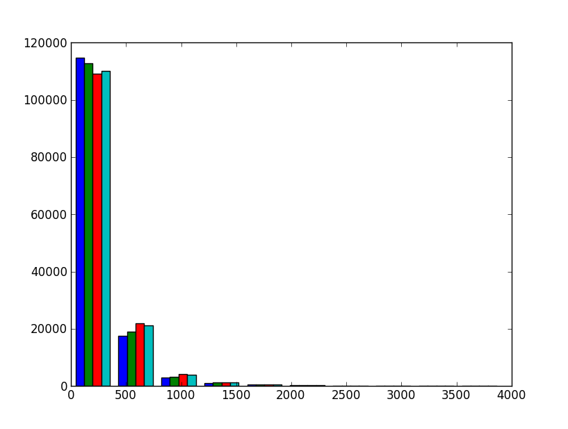
This will not do. Firstly, data from the four detectors is pictured as four side-by-side colored bars. Secondly, the number of bins is very low; it is only ten. Thirdly, the data range continues up to very high values with hardly any events.

To fix this, we’ll make use of several arguments that can be passed to the hist function. We’ll also make use of some NumPy (documentation) functionality. For Pylab documentation, see the Matplotlib site. Try this:

>>> bins = linspace(0, 2000, 101)
>>> hist(ph, bins, histtype='step', log=True)
>>> xlabel("Pulseheight [ADC]")
>>> ylabel("Counts")
>>> title("Pulseheight histogram (log scale)")

The linspace function returns an array with range from 0 to 2000 with a total number of 101 values. The first value is 0, the last is 2000. These are the edges of the bins. So, 101 values means exactly 100 bins between 0 and 2000. The hist function will then plot a stepped histogram with a log scale. Finally, we add some labels and a title. This is the result:

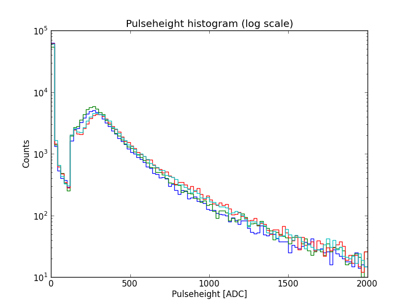
In this plot, the gamma and charged particle part of the spectrum are easy to distinguish. The cut at 123 ADC is due to the trigger. The bump at approximately 300 ADC is the so-called MIP (minimum ionizing particle) peak. For an explanation of this plot and the features of the pulseheight histogram, see David’s thesis, page 44–45, and 49–51.

Obtaining coincidences

If you work with HiSPARC data, invariably you’ll be interested in coincidences between HiSPARC stations. That is, are there showers which have been observed by multiple stations? To find out, we’ll make use of the sapphire.analysis.coincidences module.

Performing the search

Consider the following script, which you can hopefully understand by now (note that the prompt (>>>) is absent, since this is a script:

import datetime

import tables

from sapphire import download_data, CoincidencesESD


STATIONS = [501, 503, 506]
START = datetime.datetime(2013, 1, 1)
END = datetime.datetime(2013, 1, 2)


if __name__ == '__main__':
    station_groups = ['/s%d' % u for u in STATIONS]

    data = tables.open_file('data.h5', 'w')
    for station, group in zip(STATIONS, station_groups):
        download_data(data, group, station, START, END)

At this point, we have downloaded data for three stations. Note that we used the sapphire.esd for downloading. Thus, we have no traces and the download is quick. Let’s see what the datafile now contains:

>>> print(data)
data.h5 (File) ''
Last modif.: 'Mon Jan 14 17:34:39 2013'
Object Tree:
/ (RootGroup) ''
/s501 (Group) 'Data group'
/s501/events (Table(70643,)) ''
/s503 (Group) 'Data group'
/s503/events (Table(34937,)) ''
/s506 (Group) 'Data group'
/s506/events (Table(68365,)) ''

It contains three groups, one for each station. To search for coincidences between these stations, we first initialize the sapphire.analysis.coincidences.CoincidencesESD class like so:

>>> coincidences = CoincidencesESD(data, '/coincidences', station_groups)

From the documentation (click on the class above the example to go to the documentation) it is clear that we have to specify the datafile (data), the destination group (/coincidences) and the groups containing the station data (station_groups). Once that’s done, there is an easy way to search for coincidences, process the events making up the coincidences, and store them in the destination group:

>>> coincidences.search_and_store_coincidences(station_numbers=STATIONS)
100%|######################################|Time: 0:00:02
100%|######################################|Time: 0:00:00

If you want to tweak the process using non-default parameters, see the module documentation (sapphire.analysis.coincidences). For now, let us turn to the results:

>>> print(data)
data.h5 (File) ''
Last modif.: 'Mon Jan 14 17:46:23 2013'
Object Tree:
/ (RootGroup) ''
/coincidences (Group) u''
/coincidences/c_index (VLArray(2184,)) ''
/coincidences/coincidences (Table(2184,)) ''
/coincidences/s_index (VLArray(3,)) ''
/s501 (Group) ''
/s501/events (Table(70643,)) ''
/s503 (Group) ''
/s503/events (Table(34937,)) ''
/s506 (Group) ''
/s506/events (Table(65935,)) ''

The new addition is the /coincidences group. It contains three tables, which are c_index, coincidences and s_index. Information about the coincidences is stored in the coincidences table. Let’s look at the columns:

column	description
id	an index number identifying the coincidence
timestamp	the unix timestamp
nanoseconds	the nanosecond part of the timestamp
ext_timestamp	the timestamp in nanoseconds
N	the number of stations taking part in the coincidence
x	compatibility reasons
y	compatibility reasons
azimuth	compatibility reasons
zenith	compatibility reasons
size	compatibility reasons
energy	compatibility reasons
s501	flag to indicate if the first station is in coincidence
s503	as previous but for second station
s506	as previous but for third station

The columns included for compatibility reasons are used by the event simulation code. In that case, the x, y columns give the position in cartesian coordinates. Furthermore, the size and energy give the so-called shower size, and zenith and azimuth contain the direction of the (simulated) shower. These are not known for certain when working with HiSPARC data, but are included nonetheless. These columns are all set to 0.0.

The c_index array is used as an index to look up the tables and individual events making up a coincidence. The second coincidence is accessed by:

>>> data.root.coincidences.coincidences[1]
(2L, 1356998460, 730384055L, 1356998460730384055L, 2, 0.0, 0.0, 0.0,
 0.0, 0.0, 0.0, True, False, True)

Remember, the indexes are zero-based. The coincidence id is also 2:

>>> data.root.coincidences.coincidences[2]['id']
2

and the number of stations participating is 2:

>>> data.root.coincidences.coincidences[2]['N']
2

To lookup the indexes of the events taking part in this coincidence, access the c_index array using the same id:

>>> data.root.coincidences.c_index[2]
array([[ 0, 40],
       [ 2, 57]], dtype=uint32)

That is, event id 40 from station 0, event id 57 from station 2 are part of this coincidence. The event observables are still stored in their original location and can be accessed using the ids. To find the location of the station group the s_index contains the paths to the station groups.:

>>> data.root.coincidences.s_index[0]
'/s501'
>>> data.get_node('/s501', 'events')[40]
(40L, 1356998460, 730384055L, 1356998460730384055L, [2, 227, 301, 2],
 [0, 1657, 3173, 0], 0.0, 0.5117999911308289, 0.9417999982833862,
 0.0, -999.0, 12.5, 57.5, -999.0, 62.5)

Downloading coincidences

Just like events or weather data for a single station the ESD provides coincidence data. This means that you can directly download coincidences from the server. In most cases this can save a lot of disc space, because only events in a coincidence will be stored.

Downloading coincidences is very similar to downloading data. First import the required packages, open a PyTables file, and specify the date/time range. With coincidences two additional options are available, first you can select which stations you want to consider. This can be all stations in the network, by not specifying any. It can be a subset of stations by listing those stations (upto 30 stations), or a cluster of stations by giving the name of the cluster.

So first import the packages:

>>> import datetime
>>> import tables
>>> from sapphire import esd

Set the date/time range:

>>> start = datetime.datetime(2012, 12, 1)
>>> end = datetime.datetime(2012, 12, 3)

Open (in this case create) a datafile:

>>> data = tables.open_file('data_coincidences.h5', 'w')

Then download the coincidences. Here we specify the cluster ‘Enschede’ to select all stations in that cluster. By setting n to 3 we require that a coincidence has at least 3 events.

>>> esd.download_coincidences(data, cluster='Enschede',
...                           start=start, end=end, n=3)

If you now look in the data file it will contain event tables for all stations with at least one event in a coincidence, and a coincidence table for the coincidence data. Just like when coincidences were searched manually:

>>> print(data)
Object Tree:
/ (RootGroup) ''
/coincidences (Group) ''
/coincidences/c_index (VLArray(776,)) ''
/coincidences/coincidences (Table(776,)) ''
/coincidences/s_index (VLArray(124,)) ''
/hisparc (Group) ''
/hisparc/cluster_enschede (Group) ''
/hisparc/cluster_enschede/station_7001 (Group) ''
/hisparc/cluster_enschede/station_7001/events (Table(776,)) ''
/hisparc/cluster_enschede/station_7002 (Group) ''
/hisparc/cluster_enschede/station_7002/events (Table(776,)) ''
/hisparc/cluster_enschede/station_7003 (Group) ''
/hisparc/cluster_enschede/station_7003/events (Table(776,)) ''

Footnotes

[1]

Unique in this table. When data is downloaded for analysis and combined with other data into one table, the event_id will be different. To uniquely define an event, use a station number / ext_timestamp combination.

Reconstructions

Reconstructing ESD Events

Assume data_s501.h5 contains events downloaded from the ESD for station 501:

>>> import tables
>>> from sapphire import ReconstructESDEvents
>>> data = tables.open_file('data_s501.h5', 'a')
>>> station_path = '/s501'  # location of the event table in datafile
>>> rec = ReconstructESDEvents(data, station_path, 501, verbose=True)
Constructed object <Station, id: 0, number: 501, cluster:
HiSPARCStations([501])> from public database.

The parameter verbose=True forces the reconstruction class to be verbose about the metadata about station layout of timing offsets that is being used. Here, a HiSPARCStations object is created which retrieves metadata from the public database.

Now let’s reconstruct the events and store the results in the datafile:

>>> rec.reconstruct_and_store()
Reading detector offsets from public database.
100%|#################################################|Time: 0:00:31
100%|#################################################|Time: 0:00:21

The reconstruction class notifies us that detector timing offsets are being retrieved from the public database. First directions are reconstructed and subsequently core positions are reconstructed.

The results are stored in the datafile in the reconstructions group:

>>> print(data.root.s501.reconstructions)
/s501/reconstructions (Table(29569,)) ''

>>> data.root.s501.reconstructions.col('zenith')
array([ nan,  nan,  nan, ...,  nan,  nan, 0.66482645], dtype=float32)

The nan values in the zenith angle array are values that cannot be reconstructed:

>>> from numpy import isnan
>>> theta = data.root.s501.reconstructions.col('zenith')
>>> theta = theta.compress(~isnan(theta))
array([ 0.59542936,  0.74284476,  0.38334498, ...,  0.41376889,
    0.07834953,  0.66482645], dtype=float32)

Reconstructing simulated events

Assume the datafile (data) contains simulated events, generated by sapphire.simulations.groundparticles.GroundParticlesSimulation. This class stores the metadata of the simulated station (cluster) in the hdf5 file, which can be read by the reconstruction class:

>>> rec = ReconstructESDEvents(data, station_path, 501, verbose=True)
Read cluster HiSPARCStations([501]) from datafile.

The class has read the station (cluster object) from the datafile. This cluster object contains both the detector locations as well as the detector timing offsets:

>>> rec.reconstruct_and_store()
Read detector offsets from cluster object.
100%|#################################################|Time: 0:00:31
100%|#################################################|Time: 0:00:21

Note that the detector (timing) offset from the datafile are used, and not the offsets from the public database.

Reconstructing ESD coinicdences

Coincidences can be reconstructed analoguous to ESD Events:

>>> import tables
>>> from sapphire import ReconstructESDCoincidences
>>> data = tables.open_file('data_s501_s502_s503.h5', 'a')
>>> rec = ReconstructESDEvents(data, verbose=True)
Constructed cluster HiSPARCStations([501, 502, 503]) from public
database.

The constructed cluster object is created from the stations in the datafile.

Reconstruct:

>>> rec.reconstruct_and_store()
Using timing offsets from public database.
100%|#################################################|Time: 0:00:31
100%|#################################################|Time: 0:00:21

Reconstructing simulated coincidences

The ReconstructESDCoincidences class can reconstruct simulated coincidences, using the cluster objects stored by the simulation class in the datafile analoguous to ReconstructESDEvents.